Customer churn is a really interesting problem. It appears to be a simple calculation, but the more you explore it the more complex it becomes. Evidence of this complexity appears in the variety of articles written on the subject, such as:
- For Entrepreneurs uses a very straightforward method of calculation, which is then used as the basis for a number of other important SaaS metrics.
- Chaotic Flow‘s SaaS metrics archive presents some very interesting questions.
- HubSpot expands the subject of churn rate into an entire e-book.
- Shopify has a great article that includes the complexities of calculating churn.
One of the best ways to understand a problem is to create a mathematical model of how it works.
The question we need to answer is: “What exactly is Churn?”
We start by defining churn as:
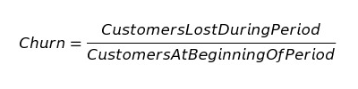
As an example, if we had 100 customers at the beginning of January, and during January, we lost 10 of those customers, our churn rate for January is 10%.
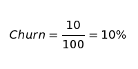
We now have a descriptive model for churn. A descriptive model summarizes what has happened but is limited if we want to understand trends in churn. With a descriptive model, the only thing we can say is, “We lost 10% of our customers this month.”
This formula implies that the following churn rates are all the same:
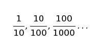
Problems with this model arise when we compare churn this month with churn last month. When comparing, we are forecasting because we are saying, “We expect to lose n% of customers next month since we lost n% this month.” Then, we use next month’s churn rate to determine whether we improve.
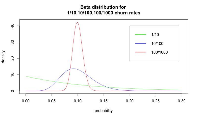
We want to compare churn between periods since it is a key performance indicator of the health of a business. To compare two time periods, we can look at churn rates as values sampled from a probability distribution.
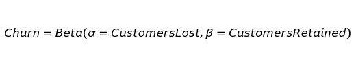
The above equation states we are looking at churn as being sampled from a beta distribution. Beta distributions model cases where the aim is to estimate the true rate of an event from its sample data.
While the mean of the distribution is the most likely value you would see, a wide range of other churn rates are potentially observable due to mere chance. The probability distribution tells us how likely those alternatives are based on the area under the curve. Although 1/10 and 100/1000 are both 10% churn rates, they represent very different distributions. Pictured below are the 1/10, 10/100, and 100/1000 churn rates visualized as distributions rather than means.
These concepts are similar in A/B tests. When you observe a churn rate of 10%, you need to have significant data to determine if it’s actually 10%.
As an example, if you have only 100 customers, and last month you lost 3%, and this month you lost 6% — it’s completely possible that your churn rate is actually the same for both months. Probability distributions allow us to determine how certain we are that our true rate of churn is reflected in the data we have collected.
With A/B testing in mind, we might be tempted to treat churn as an A/B test and collect more data to overcome uncertainty. When we run an A/B test, if we don’t have enough data to determine a winning variant, we can collect more data until we reach our desired certainty. The assumption is that the conversion rate for variant A and variant B remain the same as we collect data. Can we do this with churn data?
A major challenge with our model is that churn rates change each month. If the true rate of churn has changed between January and February, we cannot use February data to get a better estimate of the churn rate for January.
We need a way to model the following:
- Observed losses, which are pulled from a beta distribution around whatever the true churn rate is.
- The churn rate as a moving target.
A final complication is that each month we’re also acquiring people, and the number of people we’re acquiring is somewhat random. If we could model new customers as a constant number, we could reduce the model to a very simple formula, but unfortunately, this is not the case.
Looking at the big picture — Modeling churn’s effects on population
Let’s take a step back and create a model that ignores the issues regarding the uncertain rate of churn we’ve raised. Rather than focus on churn in isolation, let’s look at a model of our customer population over time. We’ll start with a simplified model, adding back in the aforementioned complexities once we have a basic understanding of how all the pieces fit together.
We have these variables:
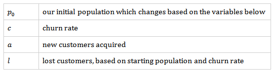
Let’s look at the formula for calculating the population in a given month.
We’ll start with calculating p1 which is the population after the first month:
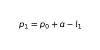
where
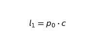
Now, let’s see what this looks like over time for the following variables:
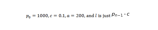
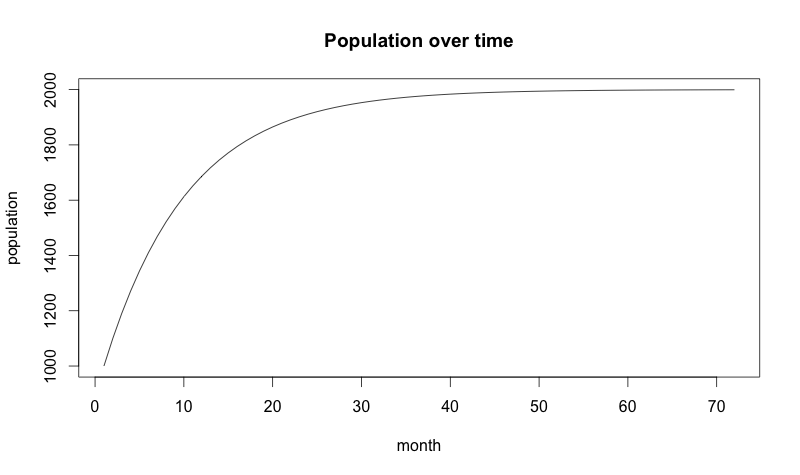
A good sanity check of any mathematical model is if the model’s description of the world reasonably matches our understanding of how the world behaves. The above plot shows growth as being much smoother than any real-world data. It also reaches a plateau in which growth stops.
This model uses constant values for churn (c) and new customers (a). In reality, neither of these values are constant. The model needs to change.
Rather than using a constant c and a, we can use a sequence of cn and an.
Let’s create a 12-month sequence of churn rates.
c = 0.1, 0.11, 0.1, 0.09, 0.085, 0.07, 0.073, 0.072, 0.07, 0.069, 0.07, 0.069
Let’s also create a sequence of new customer acquisitions for the same period.
a = 200, 180, 210, 212, 230, 250, 240, 230, 245, 250, 255, 260
These numbers model a year where churn went down and customer acquisition went up.
Our formula to calculate pn is now:
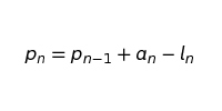
where
Remember that po is our initial starting population. For a calendar year, p1 would represent the population at the end of January.
The following chart shows what the modeled year looks like:
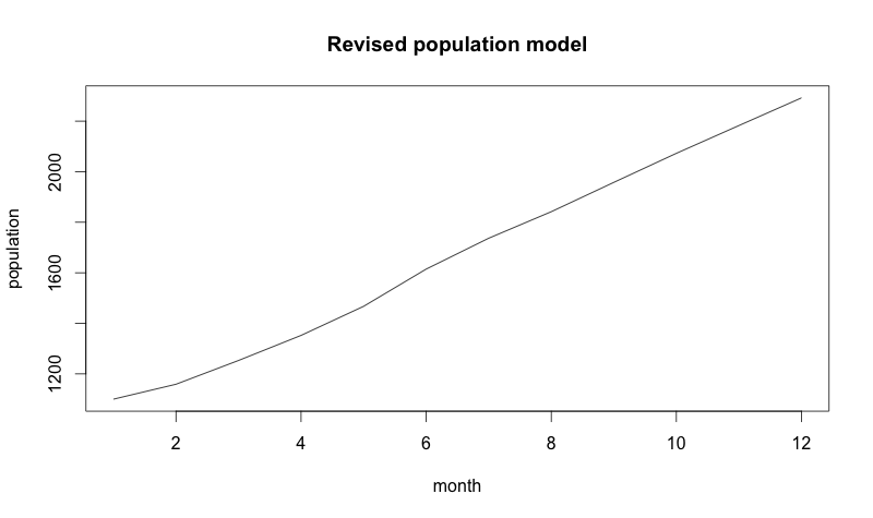
Now, that was a good year!
But another issue arises. There is a lot of uncertainty that isn’t modeled here. Let’s move to our final refinement by adding noise and a few stochastic processes.
A note on stochastic processes
The word stochastic is mathematician speak for random. A stochastic process is any process that moves randomly. The most common stochastic process is Brownian motion. If you look up Brownian motion on Wikipedia, you’ll encounter some terrifying equations, but the idea is profoundly simple.
First, we start with a normal distribution. A normal distribution is defined by its mean, μ (the model’s center), and its standard deviation, σ (how wide the model is).
A normal distribution with μ = 0 and σ= 1 looks like this:
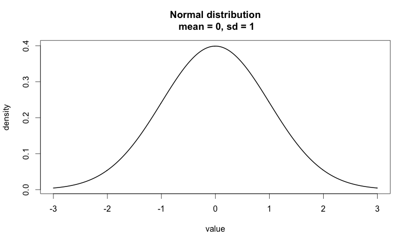
Sampling from a normal distribution means picking random numbers from the model. The closer a number is to the big bump in the middle, the more likely we are to get that number.
If we sample from N (0,1) — notation for a normal distribution with a mean of 0 and a standard deviation of 1 — 1000 times and plot the data, we get the following plot:
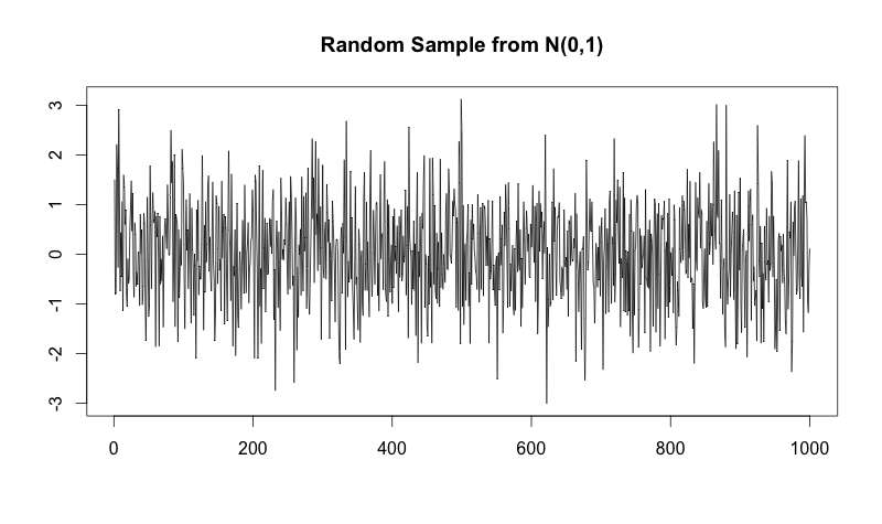
To transform this noisy sample into Brownian motion, we take the cumulative sum of the sample. Taking the cumulative sum means that each point in the Brownian motion is the sum of all the previous points in the sample.
Here’s what the exact sample above looks like when we plot it as a Brownian motion:
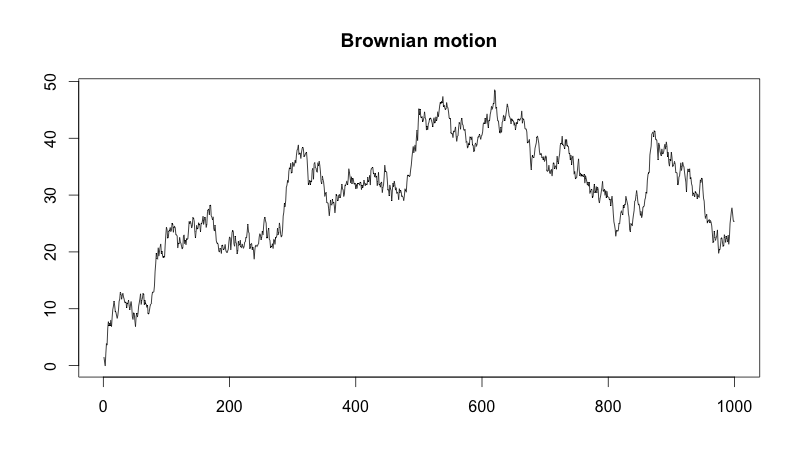
Although our samples look like noise, when we plot the cumulative sum, it looks like the movements of a stock price! In fact, Brownian motion is an essential component of the Black-Scholes model used in options pricing. Who knew trying to understand churn would lead us all the way to the world of quantitative finance?
Finally, it is essential to note that if the normal distribution we’re using has a mean greater than zero, our Brownian motion model will have a tendency to move upward. If it has a mean less than zero, it will tend to move downward. This movement is called drift because the random process is drifting a certain direction.
Building our stochastic model of customer population
Now we’re going to build a stochastic difference equation. Equations usually return a single value (algebra) or a function (differential equation). A stochastic difference equation is different. It returns a stochastic process! This makes sense when you think about it.
We are taking the stochastic processes used to describe churn and acquisition, and we are putting them together to come up with another stochastic process that represents the changes to our population of customers over time. To better understand this process, let’s look at the acquisition component of our model.
We’ll define customer acquisition as Brownian motion with a mean of μacq and a standard deviation of σacq
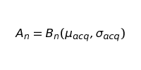
This formula says that our customer acquisition at period n is equal to the nth step in the Brownian motion we are defining with a specific mean and standard deviation (later on, we’ll touch on how we can estimate μacq and σacq). The tricky part about this is realizing that the nth step in Brownian motion is a space of many possibilities and not simply a single value.
Simulating churn is a bit more involved. Just as with customer acquisition, we’ll start by using Brownian motion as the basis for our model.
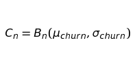
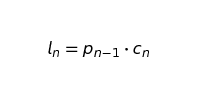
This equation models only our moving churn rate, which we can never directly observe. Another step must be added to accurately represent loss. Our loss is a random sampling from a beta distribution with the current value of Cn as the mean.
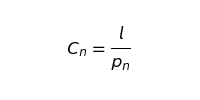
Solving for l
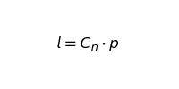
And so our loss function is
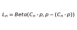
so finally we get
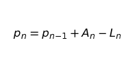
This is our stochastic difference equation. We can see that, once we have tucked away all the Brownian motion behind some symbols, we end up with a formula that is very similar to our last one. The key difference is that An and Ln represent stochastic processes at a point n rather than fixed values in a sequence.
Let’s see what the results of a single sampling from this process look like. All we need is some values to assign to our parameters.
μchurn = 0.001, σchurn = 0.001
μacq = 0.05, σacq = 40
p0 = 1000
We’re assuming that the starting value for churn is 0.1 and acquisition is 200 (meaning that our churn rate at the beginning is 10% and we’re getting 200 new customers). The image below is a single sample path from the stochastic process we defined over the period of 72 months.
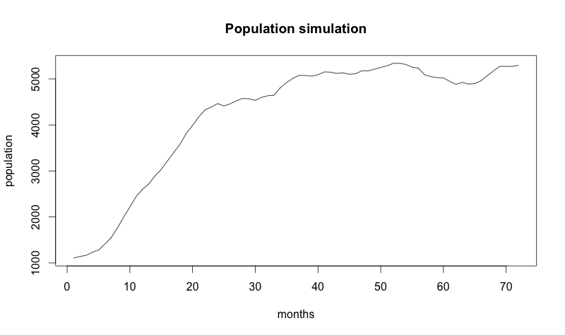
But don’t forget: now we have a stochastic model, so every time we run it, we get a different answer!
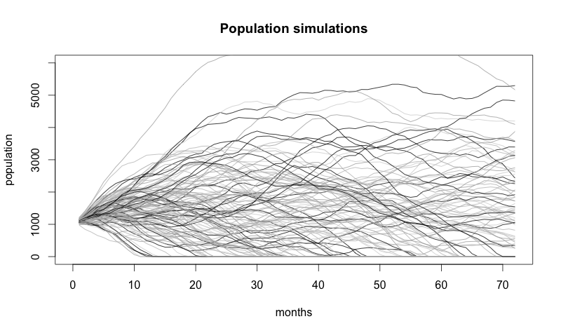
Above are the random paths that 120 very similar companies might have taken.
At this point, you might be thinking “My company is not random! We aren’t just rolling dice all day!” Stochastic models don’t claim things are random; they claim things are uncertain.
For example, every time you determine the winner of an A/B test, there is a chance your decision is wrong. Even if you run tests to 99.999% certainty, other things are out of your control. For example, there could have been a major outage in service that you couldn’t have planned for, or a popular blog could have published a piece on your company that sent more new customers than expected.
Minor fluctuations are more common than major ones, and a normal distribution accounts for this. In addition, a normal distribution with a drift accounts for your product team always improving the product and your marketing team always increasing conversions.
Modeling observed data
We are still missing the parameters for the two Brownian motion functions we have in the model: μchurn, σchurn, μacq, σacq
Remember, we can think of μ as the general tendency of churn and acquisition (ideally churn would tend to go down and acquisition up), and we can think of σ as the amount of uncertainty we face.
We can use the previous values we assumed for churn and acquisition:
c = 0.1, 0.11, 0.1, 0.09, 0.085, 0.07, 0.073, 0.072, 0.07, 0.069, 0.07, 0.069
a = 200, 180, 210, 212, 230, 250, 240, 230, 245, 250, 255, 260
Then, we use the summary statistics from these to estimate the μ and σ for our models. Our model assumes a cumulative sum of output from normal distribution. We cannot simply take the mean and standard deviations of these values. Rather, we must look at the difference between each step (this effectively undoes the summing we did previously):
cdiff = 0.010, -0.010, -0.010, -0.005, -0.015, 0.003, -0.001, -0.002, -0.001, 0.001, -0.001
adiff = -20, 30, 2, 18, 20, -10, -10, 15, 5, 5, 5
Assuming this data comes from a normal distribution, we can use the following formulae to calculate mean and standard deviation:
Calculating our churn values, we get:
μchurn = -0.002818182
σchurn = 0.006925578
and for acquisition values, we get:
μacq = 5.454545
μacq = 5.454545
A careful reader may notice that we cheated a bit in the above calculation for churn. Our calculation assumes we observed the actual churn rate. If we look at our model, we never get to observe this directly! There is always some noise added by randomly sampling from the Beta distribution.
If we make some simplifying assumptions about the beta distribution, we can solve this problem. However, for the sake of brevity, we’ll pretend we can see those churn rates.
Let’s go back to our simulation, and this time we’ll use the parameters we arrived at empirically.
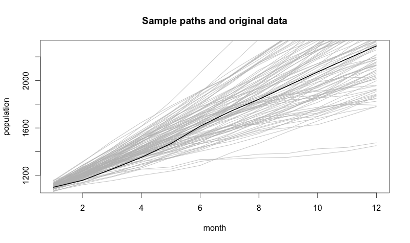
In the chart above, the dark line in the middle is our original data — the data our model is based on. The fact that our original data is in the middle of all these samples is a good sanity check since we used this data as what our expected data should be. The sample paths that diverge from it are progressively less expected could-have-beens.
Another important thing to observe about this data is that, as we move forward in time, the range of possible future populations becomes wider. The further ahead we look, the less certain we become about what the future might look like.
Using our model — The takeaway
Boards of Directors don’t usually want you to show them a stochastic process and say “Look at how much we don’t know! Isn’t that amazing?” We’ve described just how complex growth can be, but what can we do with this model?
Reviewing the many different papers on churn at the beginning of this article, you can see the practical implications of choosing one model for a metric over another. If you are uncertain what the real pros and cons are of using any particular method to calculate a metric, you can try it on simulated data and see what happens now that you are omniscient.
We also can use our knowledge of the past to attempt to gain insight into the future. Using the 12 months of data, we can see what futures that model predicts 6 months out:
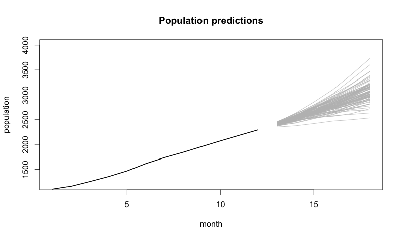
If the CEO wants to see our imaginary company reach 4000 customers, our simulation shows that we aren’t going to get there by luck. Our stochastic model gives us futures that depend on us doing everything the same as we did in the period we used to estimate our parameters. To reach 4000 customers in 6 months, this model tells us we have to change how we’re doing things.
The model also tells us that if we keep doing things the way we are, then our future looks bright. Even our worst-case predictions look good! However, all changes involve risk. So if the CEO’s goal is to reach 2500 customers in 6 months, it probably isn’t worth the risk to radically change how things are done.
We also can predict how likely certain futures are. If we simulate 1000 sample paths, how many end up above 3000 after 6 months? How likely is it that in 6 months, due to a string of mistakes, we end up with fewer customers than today?
Conclusion
Modeling churn is difficult because there is inherent uncertainty when measuring churn. This uncertainty does not change churn’s status as an essential SaaS metric. What this uncertainty does change is how we utilize churn metrics.
For any metric you use to calculate churn, make sure you understand its limitations. The smaller the number of customers you have, the more likely month-to-month churn may appear to move up or down based solely on chance. If you have a large number of customers, measuring quarterly and annual churn rates can give very different results depending on how churn is calculated and how much the true rate of churn changes during the longer period. Despite answering a simple question, churn is a complicated metric.
About the Author: Will Kurt is a Data Scientist. You can reach out to him on twitter @willkurt and see what he’s hacking on at github.com/willkurt.
Comments (12)